Back to Mathematics syllabus

Normal Distribution

CSCA Normal Distribution study guide organized around the publicly available CSCA syllabus. Practice Mathematics questions on aicsca.com.

Before planning this topic, check the CSCA Exam Guide 2026 for exam dates, registration, fees, and subject requirements.

Syllabus Alignment

This study guide is organized around the publicly available CSCA syllabus for international undergraduate applicants.

Who It Is For

International students preparing for CSCA Math, Physics, Chemistry, or Chinese exams.

Related Practice

CSCA Practice · Go to questions

Past papers and worked video solutions · Timed mock exams · All subject video lessons

Practice by Topic

Jump from this tutorial to filtered practice questions for the same knowledge point.

Tutorial Content

Normal Distribution

1. Core Concepts and Graph Features

The **Normal Distribution** (or Gaussian Distribution) is the most important continuous distribution. Its probability density curve is **Bell-shaped**. It is denoted as $X \sim N(\mu, \sigma^2)$.

* **Mean ($\mu$)**: Determines the **central location** of the curve. The curve is symmetric about $x = \mu$.

* **Standard Deviation ($\sigma$)**: Determines the **shape (width)** of the curve. A larger $\sigma$ means more dispersed data (flatter curve); a smaller $\sigma$ means more concentrated data (steeper curve).

2. The Empirical Rule (3σ Rule)

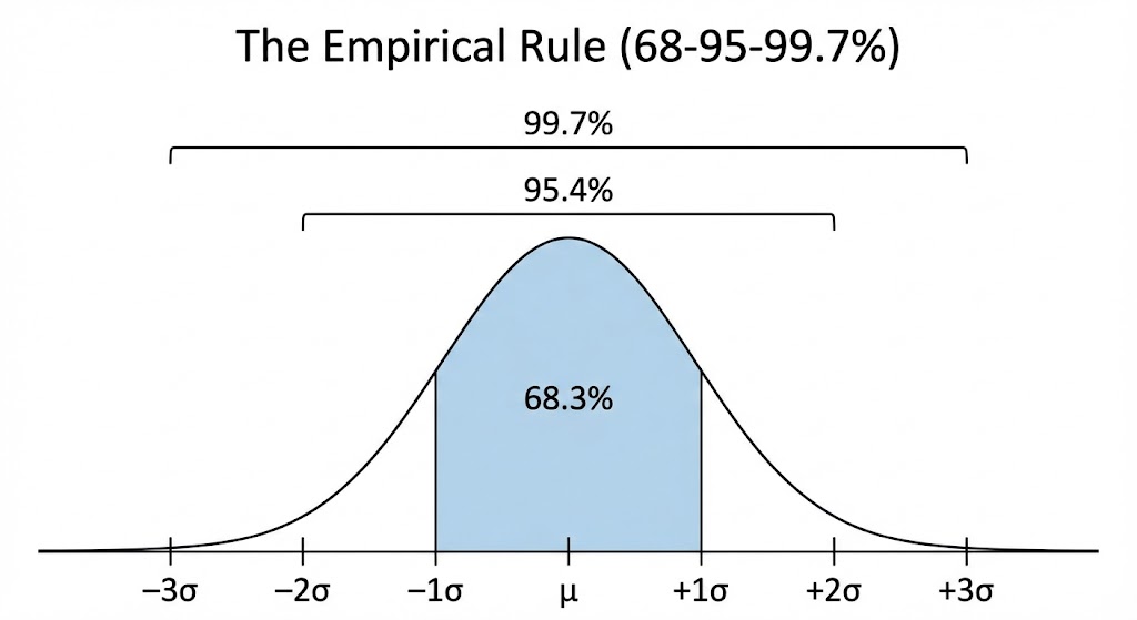
In a normal distribution, the probability of data falling around the mean is constant. This is a high-frequency topic in the CSCA exam. Memorize these values:

* $(\mu - \sigma, \mu + \sigma)$: Covers approx. **68.3%** of the data.

* $(\mu - 2\sigma, \mu + 2\sigma)$: Covers approx. **95.4%** of the data.

* $(\mu - 3\sigma, \mu + 3\sigma)$: Covers approx. **99.7%** of the data.

This implies that almost all data points lie within 3 standard deviations of the mean.

3. Standardization and Z-Score

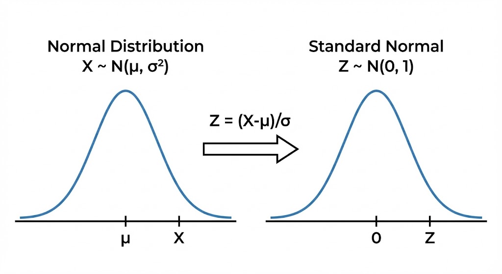
To calculate probabilities for any normal distribution, we transform it into the **Standard Normal Distribution** $N(0, 1)$, which has a mean of 0 and a variance of 1.

**Transformation Formula (Z-Score)**:

$$Z = \frac{X - \mu}{\sigma}$$

* **Meaning**: The $Z$-score represents how many standard deviations the raw data $X$ is away from the mean $\mu$.

* **Application**: Once converted to a $Z$-score, we can use the Standard Normal Table to find probabilities.

Typical Example

**Problem**: Exam scores follow a normal distribution $N(70, 100)$ (Note: $100$ is variance $\sigma^2$, so $\sigma=10$). Find the probability that a score is between 60 and 80.

**Solution**:

1. **Standardize**: Convert $X=60$ and $X=80$ into $Z$ values.

$$Z_1 = \frac{60-70}{10} = -1, \quad Z_2 = \frac{80-70}{10} = 1$$

2. **Use Symmetry/Rule**:

$$P(60 < X < 80) = P(-1 < Z < 1)$$

According to the Empirical Rule, the area within 1 standard deviation of the mean is approx. **68.3%**.